Harmonization of Multi-Site Data

When brain images are acquired at different sites or on different scanners, the resulting scalar measurements contain site-specific technical biases that can mask or mimic real biological effects. ComBat removes these additive and multiplicative site effects while preserving biological covariates like age and sex.

This notebook demonstrates the harmonize_volumes function on synthetic data with known site biases and a known age effect.

Pipeline overview

1. Generate synthetic multi-site scalar maps with known biases

2. Visualize site effects before harmonization

3. Run ComBat harmonization

4. Compare before and after

5. Verify that the biological (age) effect is preserved

1. Generate synthetic multi-site data

We create synthetic scalar volumes for 3 “sites” with 8 subjects each. Each site has a different additive shift and multiplicative scale applied on top of a shared biological signal (a smooth gradient + age effect).

import matplotlib.pyplot as plt
import numpy as np
import pandas as pd

from kwneuro.resource import InMemoryVolumeResource

rng = np.random.default_rng(123)
shape = (30, 36, 20)
n_per_site = 8
sites = ["Scanner_A", "Scanner_B", "Scanner_C"]

# Smooth base signal (shared biology)
x = np.linspace(0.2, 0.8, shape[0])[:, None, None]
y = np.linspace(0.3, 0.6, shape[1])[None, :, None]
base = x * y * np.ones(shape)

# Site-specific biases
site_params = {
    "Scanner_A": {"shift": 0.0, "scale": 1.0},
    "Scanner_B": {"shift": 0.15, "scale": 1.4},
    "Scanner_C": {"shift": -0.1, "scale": 0.7},
}

# Brain mask
mask_array = np.zeros(shape, dtype=np.int8)
mask_array[4:26, 4:32, 3:17] = 1
mask = InMemoryVolumeResource(array=mask_array, affine=np.eye(4), metadata={})

# Generate volumes
volumes = []
site_labels = []
ages = []

for site in sites:
    p = site_params[site]
    for _ in range(n_per_site):
        age = rng.uniform(25, 75)
        age_effect = age * 0.002
        noise = rng.normal(0, 0.015, shape)
        vol_data = (base + age_effect + noise) * p["scale"] + p["shift"]
        volumes.append(InMemoryVolumeResource(
            array=vol_data, affine=np.eye(4), metadata={}
        ))
        site_labels.append(site)
        ages.append(age)

covars = pd.DataFrame({"site": site_labels, "age": ages})
print(f"Generated {len(volumes)} volumes across {len(sites)} sites")
print(covars.groupby("site")["age"].describe()[["count", "mean", "std"]])

Generated 24 volumes across 3 sites
           count       mean        std
site
Scanner_A    8.0  54.924903  15.648836
Scanner_B    8.0  57.283493  12.979633
Scanner_C    8.0  52.865805  12.695440

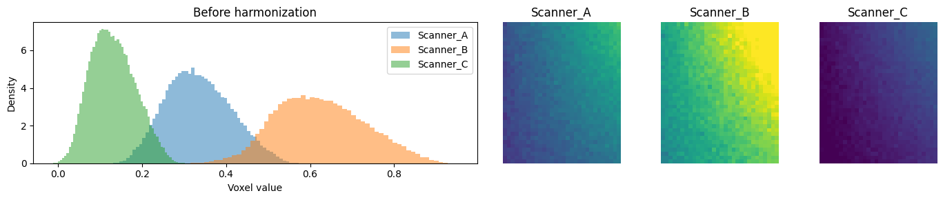
2. Visualize site effects before harmonization

Each site’s voxel-value distribution is shifted and scaled differently.

mask_idx = np.nonzero(mask_array > 0)
mid_slice = shape[2] // 2

fig, axes = plt.subplots(1, 4, figsize=(14, 3), width_ratios=[3, 1, 1, 1])

# Histograms
for site, color in zip(sites, ["tab:blue", "tab:orange", "tab:green"]):
    site_voxels = []
    for vol, s in zip(volumes, site_labels):
        if s == site:
            site_voxels.append(vol.get_array()[mask_idx])
    all_voxels = np.concatenate(site_voxels)
    axes[0].hist(all_voxels, bins=60, alpha=0.5, label=site, color=color, density=True)

axes[0].set_xlabel("Voxel value")
axes[0].set_ylabel("Density")
axes[0].set_title("Before harmonization")
axes[0].legend()

# Example slices (one subject per site, shared color range)
all_masked = np.concatenate([v.get_array()[mask_idx] for v in volumes])
vmin, vmax = np.percentile(all_masked, [1, 99])
for i, site in enumerate(sites):
    idx = site_labels.index(site)
    arr = volumes[idx].get_array()[:, :, mid_slice]
    axes[i + 1].imshow(arr.T, cmap="viridis", origin="lower", vmin=vmin, vmax=vmax)
    axes[i + 1].set_title(site)
    axes[i + 1].axis("off")

plt.tight_layout()
plt.show()

3. Run ComBat harmonization

from kwneuro.harmonize import harmonize_volumes

harmonized, estimates = harmonize_volumes(
    volumes,
    covars,
    batch_col="site",
    mask=mask,
    continuous_cols=["age"],
)

print(f"Harmonized {len(harmonized)} volumes")

[neuroCombat] Creating design matrix
[neuroCombat] Standardizing data across features
[neuroCombat] Fitting L/S model and finding priors
[neuroCombat] Finding parametric adjustments
[neuroCombat] Final adjustment of data
Harmonized 24 volumes

4. Compare before and after

After harmonization, the per-site distributions should overlap.

fig, axes = plt.subplots(1, 4, figsize=(14, 3), width_ratios=[3, 1, 1, 1])

for site, color in zip(sites, ["tab:blue", "tab:orange", "tab:green"]):
    site_voxels = []
    for vol, s in zip(harmonized, site_labels):
        if s == site:
            site_voxels.append(vol.get_array()[mask_idx])
    all_voxels = np.concatenate(site_voxels)
    axes[0].hist(all_voxels, bins=60, alpha=0.5, label=site, color=color, density=True)

axes[0].set_xlabel("Voxel value")
axes[0].set_ylabel("Density")
axes[0].set_title("After harmonization")
axes[0].legend()

# Use same color range as the "before" plot for comparison
for i, site in enumerate(sites):
    idx = site_labels.index(site)
    arr = harmonized[idx].get_array()[:, :, mid_slice]
    axes[i + 1].imshow(arr.T, cmap="viridis", origin="lower", vmin=vmin, vmax=vmax)
    axes[i + 1].set_title(site)
    axes[i + 1].axis("off")

plt.tight_layout()
plt.show()

# Print site means
print("Per-site mean voxel values:")
for site in sites:
    before_means = [
        v.get_array()[mask_idx].mean()
        for v, s in zip(volumes, site_labels)
        if s == site
    ]
    after_means = [
        v.get_array()[mask_idx].mean()
        for v, s in zip(harmonized, site_labels)
        if s == site
    ]
    print(
        f"  {site:12s}  before: {np.mean(before_means):.4f}  "
        f"after: {np.mean(after_means):.4f}"
    )

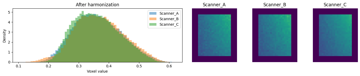
Per-site mean voxel values:
  Scanner_A     before: 0.3348  after: 0.3640
  Scanner_B     before: 0.6254  after: 0.3685
  Scanner_C     before: 0.1315  after: 0.3595

5. Verify covariate preservation

The age effect should survive harmonization. We check the correlation between age and mean voxel intensity before and after.

means_before = [v.get_array()[mask_idx].mean() for v in volumes]
means_after = [v.get_array()[mask_idx].mean() for v in harmonized]

corr_before = np.corrcoef(ages, means_before)[0, 1]
corr_after = np.corrcoef(ages, means_after)[0, 1]

fig, axes = plt.subplots(1, 2, figsize=(12, 4), sharey=True)

for site, color in zip(sites, ["tab:blue", "tab:orange", "tab:green"]):
    mask_s = [s == site for s in site_labels]
    site_ages = [a for a, m in zip(ages, mask_s) if m]
    site_before = [m for m, s in zip(means_before, mask_s) if s]
    site_after = [m for m, s in zip(means_after, mask_s) if s]
    axes[0].scatter(site_ages, site_before, label=site, color=color, s=50)
    axes[1].scatter(site_ages, site_after, label=site, color=color, s=50)

axes[0].set_xlabel("Age")
axes[0].set_ylabel("Mean voxel value")
axes[0].set_title(f"Before (r = {corr_before:.3f})")
axes[0].legend()

axes[1].set_xlabel("Age")
axes[1].set_title(f"After (r = {corr_after:.3f})")
axes[1].legend()

plt.suptitle("Age vs. mean voxel value")
plt.tight_layout()
plt.show()

print(f"Age correlation before: {corr_before:.4f}")
print(f"Age correlation after:  {corr_after:.4f}")

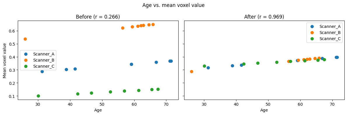
Age correlation before: 0.2661
Age correlation after:  0.9691